Building Blocks for Deep Learning: Crafting an MLP with Triton

14 minute read

Published: December 26, 2024

In our previous post, we dipped our toes into the world of Triton by writing simple custom kernels. We learned how to add a scalar to a tensor and perform element-wise multiplication, understanding the fundamental concepts of launching kernels and managing GPU memory.

Now, we’re ready to take things up a notch. In this blog post, we’ll leverage our newfound knowledge to build the fundamental components of a deep learning model: a Multilayer Perceptron (MLP). Specifically, we’ll focus on implementing matrix multiplication and activation functions using Triton, the workhorses behind most neural network computations.

From Kernels to Neural Networks: The Power of Customization

Why go through the effort of writing these core operations ourselves when libraries like PyTorch already provide highly optimized implementations? The answer lies in the potential for further performance gains and the ability to deeply understand and customize the inner workings of our models. By crafting these building blocks with Triton, we gain fine-grained control and can potentially unlock even better performance tailored to our specific needs and hardware.

The Core Operation: Matrix Multiplication in Triton

Matrix multiplication is at the heart of most deep learning models. It’s the operation that allows layers in a neural network to transform input data into more meaningful representations. Optimizing matrix multiplication is crucial for achieving good performance, especially for large models.

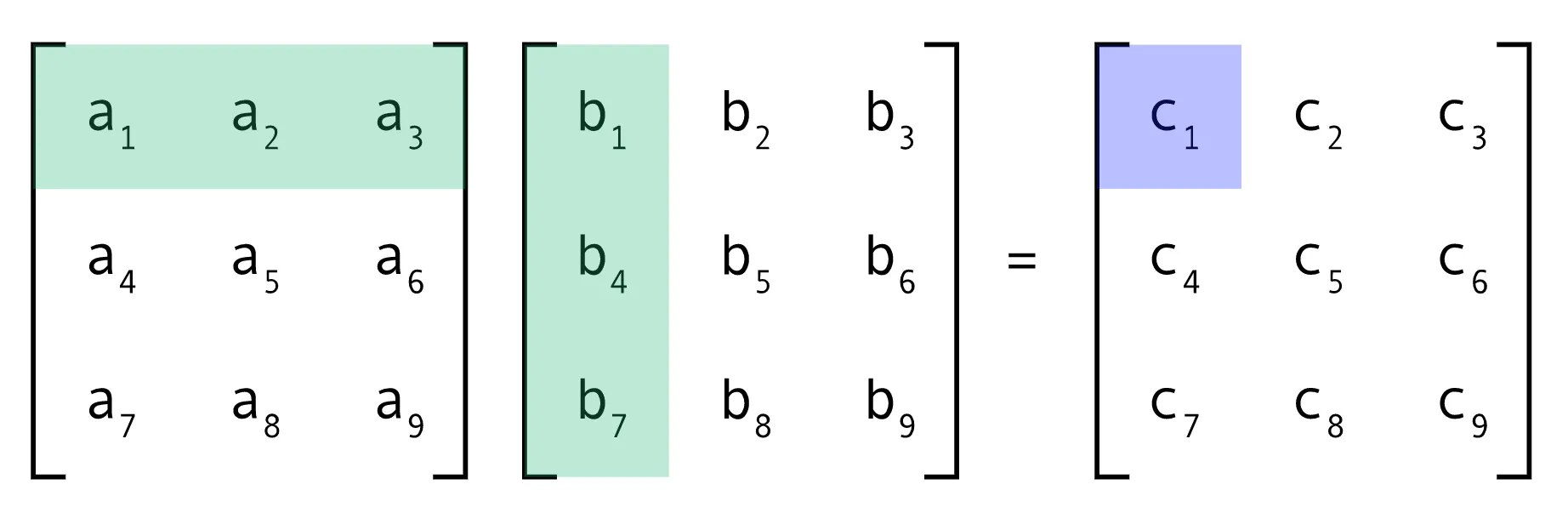
In our previous post, we dealt with element-wise operations. Matrix multiplication is more complex as it involves combining elements from two matrices in a specific way. If you recall from linear algebra, to get the element at row i and column j of the resulting matrix C (from multiplying A and B), you need to take the dot product of the i-th row of A and the j-th column of B.

Matrix Multiplication. Credit: @Charchithowitzer

Tiling for Efficiency

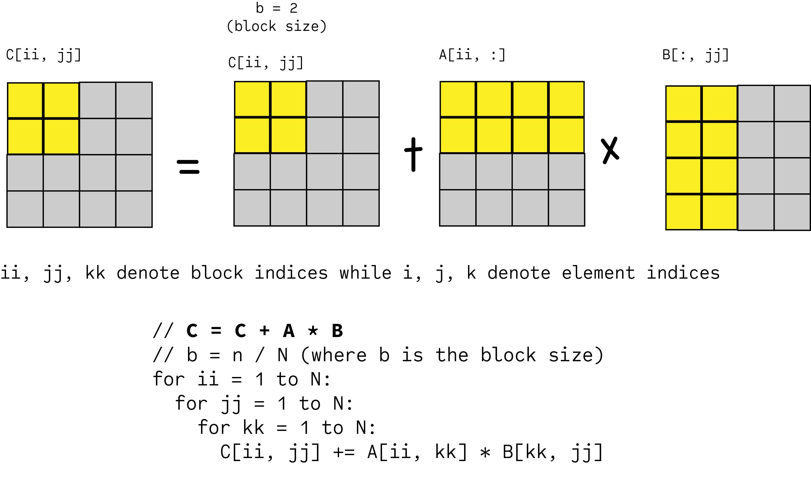
A naive implementation of matrix multiplication using nested loops can be inefficient on GPUs. To maximize performance, we often use a technique called tiling or blocking. The idea is to divide the matrices into smaller blocks and perform the multiplication on these blocks. This improves data locality, allowing the GPU to access the necessary data more quickly and efficiently.

Matrix Multiplication. Credit: @Malith Jayaweera

Let’s revisit the Triton kernel for batched matrix multiplication (BMM), which is commonly used in deep learning. First, let’s look at the pseudocode to understand the logic:

Kernel: bmm_kernel(output, input1, input2, ...)

  // Get the batch ID and the ID for this matrix multiplication instance
  batch_id = get_current_batch_id()
  program_id = get_current_program_id()

  // Calculate the block indices for this instance
  block_row_index = calculate_block_row_index(program_id)
  block_col_index = calculate_block_col_index(program_id)

  // Calculate the row and column offsets for this block
  row_offsets = calculate_row_offsets(block_row_index)
  col_offsets = calculate_col_offsets(block_col_index)
  inner_offsets = calculate_inner_offsets()

  // Initialize the output block to zeros
  output_block = zeros()

  // Loop through the inner dimension (K) in blocks
  for k_block_start in inner_dimension_blocks:
    // Calculate pointers to the input blocks
    input1_ptrs = get_input1_block_pointers(row_offsets, inner_offsets, batch_id, k_block_start)
    input2_ptrs = get_input2_block_pointers(inner_offsets, col_offsets, batch_id, k_block_start)

    // Load the input blocks
    input1_block = load_from_memory(input1_ptrs)
    input2_block = load_from_memory(input2_ptrs)

    // Perform matrix multiplication on the blocks
    intermediate_result = matrix_multiply(input1_block, input2_block)

    // Accumulate the results
    output_block += intermediate_result

  // Calculate the output pointers
  output_ptrs = get_output_block_pointers(row_offsets, col_offsets, batch_id)

  // Store the output block to memory
  store_to_memory(output_ptrs, output_block)

This pseudocode illustrates the core idea of dividing the matrices into blocks and performing the multiplication on these blocks in a loop. Now, here’s the actual Triton kernel:

import torch
import triton
import triton.language as tl

@triton.autotune(
    configs=[
        triton.Config({'BLOCK_SIZE_M': 128, 'BLOCK_SIZE_N': 128, 'BLOCK_SIZE_K': 32, 'GROUP_SIZE_M': 8}),
        triton.Config({'BLOCK_SIZE_M': 64,  'BLOCK_SIZE_N': 64,  'BLOCK_SIZE_K': 32, 'GROUP_SIZE_M': 8}),
        triton.Config({'BLOCK_SIZE_M': 32,  'BLOCK_SIZE_N': 32,  'BLOCK_SIZE_K': 16, 'GROUP_SIZE_M': 8}),
    ],
    key=['M', 'N', 'K'],
)
@triton.jit
def bmm_kernel(
    x_ptr, y_ptr, o_ptr,
    M, N, K,
    stride_al, stride_am, stride_ak,
    stride_bl, stride_bk, stride_bn,
    stride_ol, stride_om, stride_on,
    BLOCK_SIZE_M: tl.constexpr,
    BLOCK_SIZE_N: tl.constexpr,
    BLOCK_SIZE_K: tl.constexpr,
    GROUP_SIZE_M: tl.constexpr,
):
    pid_batch = tl.program_id(0)
    pid = tl.program_id(1)

    num_pid_m = tl.cdiv(M, BLOCK_SIZE_M)
    num_pid_n = tl.cdiv(N, BLOCK_SIZE_N)
    num_pid_in_group = GROUP_SIZE_M * num_pid_n
    group_id = pid // num_pid_in_group
    first_pid_m = group_id * GROUP_SIZE_M
    group_size_m = min(num_pid_m - first_pid_m, GROUP_SIZE_M)
    pid_m = first_pid_m + (pid % group_size_m)
    pid_n = (pid % num_pid_in_group) // group_size_m

    offs_am = pid_m * BLOCK_SIZE_M + tl.arange(0, BLOCK_SIZE_M)
    offs_bn = pid_n * BLOCK_SIZE_N + tl.arange(0, BLOCK_SIZE_N)
    offs_k = tl.arange(0, BLOCK_SIZE_K)

    x_ptrs = x_ptr + (offs_am[:, None] * stride_am + offs_k[None, :] * stride_ak + pid_batch * stride_al)
    y_ptrs = y_ptr + (offs_k[:, None] * stride_bk + offs_bn[None, :] * stride_bn + pid_batch * stride_bl)

    o = tl.zeros((BLOCK_SIZE_M, BLOCK_SIZE_N), dtype=tl.float32)

    for k in range(0, K, BLOCK_SIZE_K):
        x = tl.load(x_ptrs, mask=offs_k[None, :] < min(BLOCK_SIZE_K, K - k), other=0.0)
        y = tl.load(y_ptrs, mask=offs_k[:, None] < min(BLOCK_SIZE_K, K - k), other=0.0)
        o += tl.dot(x, y)

        x_ptrs += BLOCK_SIZE_K * stride_ak
        y_ptrs += BLOCK_SIZE_K * stride_bk

    offs_m = pid_m * BLOCK_SIZE_M + tl.arange(0, BLOCK_SIZE_M)
    offs_n = pid_n * BLOCK_SIZE_N + tl.arange(0, BLOCK_SIZE_N)
    mask = (offs_m[:, None] < M) & (offs_n[None, :] < N)

    o_ptrs = o_ptr + stride_om * offs_m[:, None] + stride_on * offs_n[None, :] + stride_ol * pid_batch
    tl.store(o_ptrs, o, mask=mask)

Let’s break down the key parts:

@triton.autotune: This powerful decorator tells Triton to try different configurations (defined in the configs list) and automatically choose the one that performs best for the given input sizes. The key argument specifies which input dimensions to consider when autotuning.
Block Sizes (BLOCK_SIZE_M, BLOCK_SIZE_N, BLOCK_SIZE_K): These constexprs define the dimensions of the blocks we’re working with, mirroring the block_size concept in the pseudocode. BLOCK_SIZE_M and BLOCK_SIZE_N relate to the output matrix’s row and column blocks, while BLOCK_SIZE_K relates to the inner dimension of the multiplication.
Program IDs and Grid Mapping: We use tl.program_id(0) and tl.program_id(1) to get the IDs for the batch and the individual matrix multiplication within the batch, corresponding to batch_id and program_id in the pseudocode. The subsequent calculations determine which block of the output matrix each program instance is responsible for.
Offsets: offs_am, offs_bn, and offs_k calculate the offsets within the input and output matrices for the current block, similar to the offset calculations in the pseudocode.
Loading Data in Blocks: tl.load is used to load blocks of x and y into registers, implementing the load_from_memory step in the pseudocode. Notice how we use masking (mask=...) to handle cases where the block might extend beyond the matrix boundaries.
tl.dot(x, y): This performs the matrix multiplication on the loaded blocks, directly corresponding to the matrix_multiply operation in the pseudocode.
Accumulation: The o += tl.dot(x, y) line accumulates the results of the block multiplications.
Storing the Output Block: tl.store writes the calculated block of the output matrix to memory, implementing the store_to_memory step.
Strides: The stride_ arguments are crucial for navigating multi-dimensional arrays in memory. They tell the kernel how many memory locations to jump to move to the next element along a specific dimension. To make this kernel callable from Python, we create a wrapper function:

def bmm(x, y):
    # ... (code from the previous blog post)
    unsqueeze = False
    if x.ndim == 2:
        x = x.unsqueeze(0)
        unsqueeze = True
    B, M, K = x.shape

    if y.ndim == 2:
        y = y.unsqueeze(0).expand(B, -1, -1)

    _, K_y, N = y.shape
    assert K == K_y, "Inner dimensions of matrices must match for multiplication."

    o = torch.empty((B, M, N), device=x.device, dtype=x.dtype)

    grid = lambda META: (B, triton.cdiv(M, META['BLOCK_SIZE_M']) * triton.cdiv(N, META['BLOCK_SIZE_N']))

    bmm_kernel[grid](
        x, y, o,
        M, N, K,
        x.stride(0), x.stride(1), x.stride(2),
        y.stride(0), y.stride(1), y.stride(2),
        o.stride(0), o.stride(1), o.stride(2),
    )

    torch.cuda.synchronize()
    if unsqueeze:
        return o.squeeze(0)
    else:
        return o

This function handles reshaping the input tensors if needed and sets up the grid size for launching the kernel. The grid lambda function calculates the appropriate number of program instances based on the block sizes determined by the autotuner.

Adding Flavor: Custom Activation Functions

Activation functions introduce non-linearity into neural networks, allowing them to learn complex patterns. While PyTorch provides a wide range of activation functions, implementing them directly within our Triton kernels can sometimes lead to performance improvements by reducing data movement between kernel calls. This is often referred to as “kernel fusion.”

Here are examples of implementing common activation functions as Triton JIT functions:

@triton.jit
def leaky_relu(x):
    return tl.where(x >= 0, x, 0.01 * x)

@triton.jit
def relu(x):
    return tl.where(x >= 0, x, 0)

@triton.jit
def squared_relu(x):
    return tl.where(x > 0, x * x, 0.)

@triton.jit
def sigmoid(x):
    return 1. / (1. + tl.exp(-x))

These are straightforward implementations using Triton’s conditional logic (tl.where) and basic mathematical operations.

To integrate these activation functions into our matrix multiplication kernel, we can add an activation parameter:

@triton.autotune(...) # Your autotune configuration
@triton.jit
def bmm_kernel(
        # ... (previous parameters)
        activation: tl.constexpr
):
    # ... (previous kernel code)

    if activation == "relu":  # ReLU
        o = relu(o)
    elif activation == "leaky_relu":  # Leaky ReLU
        o = leaky_relu(o)
    elif activation == "squared_relu":  # Squared ReLU
        o = squared_relu(o)
    elif activation == "sigmoid":  # Sigmoid
        o = sigmoid(o)

    # ... (rest of the kernel code)

The activation: tl.constexpr parameter allows us to pass the activation function name as a compile-time constant. Inside the kernel, we use conditional statements to apply the selected activation function.

We also need to modify the bmm Python wrapper to accept the activation function as an argument:

def bmm(x, y, activation=None):
    # ... (rest of the bmm function, passing 'activation' to the kernel)
    bmm_kernel[grid](
        # ... (previous arguments)
        activation=activation,
    )

Building the Linear Layer

Now that we have our custom matrix multiplication and activation functions, we can combine them to create a linear layer, the fundamental building block of an MLP. To integrate our Triton kernels with PyTorch’s automatic differentiation, we use torch.autograd.Function:

from torch.autograd import Function

class ActivationFusedBatchMatrixMultiplicationFn(Function):

    @staticmethod
    def forward(ctx, x, y, activation=None):
        out = bmm(x, y, activation)
        if x.requires_grad or y.requires_grad:
            ctx.save_for_backward(x, y, out)
            ctx.activation = activation
        return out

    @staticmethod
    def backward(ctx, grad_output):
        x, y, out = ctx.saved_tensors
        activation = ctx.activation

        # Calculate the gradient of the activation function
        if activation == 'relu':
            mask = (out > 0)
            grad_z = grad_output * mask
        elif activation == 'leaky_relu':
            mask = (out >= 0)
            grad_z = grad_output * mask + 0.01 * grad_output * (~mask)
        elif activation == 'squared_relu':
            mask = (out > 0)
            grad_z = grad_output * (2.0 * torch.sqrt(out) * mask)
        elif activation == 'sigmoid':
            grad_z = grad_output * out * (1.0 - out)
        else:
            grad_z = grad_output

        dx = bmm(grad_z, y.transpose(-2, -1))
        dw = bmm(x.transpose(-2, -1), grad_z)

        return dx, dw, None

class LinearLayerTriton(nn.Module):
    def __init__(self, in_features, out_features, activation=None):
        super().__init__()
        self.weight = nn.Parameter(torch.empty(out_features, in_features, device='cuda'))
        self.bias = nn.Parameter(torch.zeros(out_features, device='cuda'))
        self.activation = activation
        nn.init.xavier_uniform_(self.weight)

    def forward(self, x):
        output = ActivationFusedBatchMatrixMultiplicationFn.apply(x, self.weight.T, self.activation)
        return output + self.bias

The ActivationFusedBatchMatrixMultiplicationFn handles both the forward and backward passes of the matrix multiplication with the fused activation. In the backward pass, we calculate the gradients based on the chosen activation function.

The LinearLayerTriton module encapsulates the matrix multiplication, bias addition, and activation function into a reusable layer.

Assembling the MLP

Before making the MLP, we need to make a wrapper for our LinearLayer to make it comparable with torch.

class LinearLayerTorch(nn.Module):
    def __init__(self, in_features, out_features, activation=None):
        super().__init__()
        self.layer = nn.Linear(in_features, out_features)
        if activation == 'relu':
            self.activation = nn.ReLU()
        elif activation == 'leaky_relu':
            self.activation = nn.LeakyReLU(0.01)
        elif activation == 'squared_relu':
            self.activation = nn.ReLU()
        elif activation == 'sigmoid':
            self.activation = nn.Sigmoid()
        else:
            self.activation = None

    def forward(self, x):
        output = self.layer(x)
        if self.activation:
            output = self.activation(output)
        return output


class LinearLayer(nn.Module):
    def __init__(self, in_features, out_features, activation=None, mode='torch'):
        super().__init__()
        if mode == 'torch':
            self.layer = LinearLayerTorch(in_features, out_features, activation)
        elif mode == 'triton':
            self.layer = LinearLayerTriton(in_features, out_features, activation)

    def forward(self, x):
        return self.layer(x)

Finally, we can create our MLP by stacking these custom linear layers:

class MLP(nn.Module):
    def __init__(self, layer_sizes, activations=None, mode='triton'):
        super(MLP, self).__init__()
        if activations is None:
            activations = [None] * (len(layer_sizes) - 1)

        assert len(layer_sizes) - 1 == len(activations), "Mismatch between layers and activations."

        self.layers = nn.ModuleList(
            [
                LinearLayer(layer_sizes[i], layer_sizes[i + 1], activations[i], mode)
                for i in range(len(layer_sizes) - 1)
            ]
        )

    def forward(self, x):
        for layer in self.layers:
            x = layer(x)
        return x

This MLP class takes a list of layer sizes and activation functions and creates a sequential model using our custom LinearLayer.

Training Our Triton-Powered MLP

With our MLP defined, we can train it just like any other PyTorch model:

import torchvision
import torchvision.transforms as transforms
import torch.nn as nn
import torch.optim as optim

# Load MNIST dataset
transform = transforms.Compose([transforms.ToTensor(), transforms.Normalize((0.5,), (0.5,))])
train_dataset = torchvision.datasets.MNIST(root='./data', train=True, download=True, transform=transform)
train_loader = torch.utils.data.DataLoader(train_dataset, batch_size=64, shuffle=True)

# Define the model
mode = 'triton'
layer_sizes = [784, 256, 128, 10]
activations = ["relu", "relu", None]
model = MLP(layer_sizes, activations, mode).to('cuda')

# Loss and optimizer
criterion = nn.CrossEntropyLoss()
optimizer = optim.Adam(model.parameters(), lr=0.001)

# Training loop
for epoch in range(5):
    losses = []
    for images, labels in train_loader:
        images = images.view(images.size(0), -1).to('cuda')
        labels = labels.to('cuda')

        # Forward pass
        outputs = model(images)
        loss = criterion(outputs, labels)
        losses.append(loss.item())
        # Backward and optimize
        optimizer.zero_grad()
        loss.backward()
        optimizer.step()
    print(f'Epoch [{epoch+1}/5] Loss: {sum(losses)/len(losses):.4f}')

Training log:

Epoch [1/5] Loss: 0.2886
Epoch [2/5] Loss: 0.1369
Epoch [3/5] Loss: 0.1061
Epoch [4/5] Loss: 0.0860
Epoch [5/5] Loss: 0.0741

Evaluation

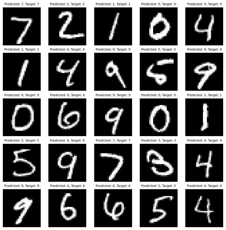
Finally, we evaluated our Triton-based MLP on the MNIST test set which exhibited 97.2% accuracy. Image below demonstrated examples of the model output in MNIST dataset. The detailed benchmarking code and performance plots are available in the GitHub repository.

Examples of Triton MLP output on MNIST.

Conclusion

In this blog post, we’ve taken a significant step forward in our Triton journey. We’ve implemented the core building blocks of an MLP – matrix multiplication and activation functions – using custom Triton kernels. We’ve seen how to leverage Triton’s autotuning capabilities and how to integrate our kernels with PyTorch’s automatic differentiation system.

By crafting these fundamental components ourselves, we gain a deeper understanding of how these operations work at a lower level and open the door for further optimization and customization. In future explorations, we can delve into more advanced kernel optimization techniques, explore different network architectures, and benchmark the performance of our Triton-powered MLP against standard PyTorch implementations. Stay tuned in the next blog, we evaluate the performance of our triton based model!

Share on

Twitter Facebook LinkedIn

Danial Kamali